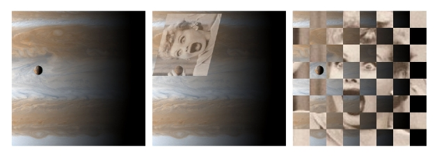
Using Images

Create a image representation for use with `show_image()`

INPUTS

  data    -- a NumPy matrix
  min_value
          -- lower bound on valid data
  max_value
          -- upper bound on valid data
  masking -- defaults to false
  max_code
          -- integer between 1 and 255 (default: 255)
  low_threshold
          -- integer between 0 and 255 (default: 0)
  high_threshold
          -- integer between 0 and 255 (default: max_code)

This method creates a data representation for use with
`show_image()` from the NumPy matrix `data`.  Data values
between `min_value` and `max_value` are mapped linearly to
numbers between 0 and `max_code` and then rounded to the
nearest integer.  Data values less than `min_value` are mapped
to the integer specied by `low_threshold`, and values greater
than `max_value` are mapped to the integer given by
`high_threshold`.

If the flag `masking` is True, then `max_code` is set to 254
and all data values out of range are assigned the code 255.
The result can then be used in a call to `show_image()` with
`value_mask` set to 255 to prevent out-of-range values from
being displayed.

Create a monochrome image representation for use with `show_image()`

INPUTS

  data    -- a NumPy matrix
  threshold
          -- defaults to 0.0
  reverse -- defaults to False

Creates a data representation suitable for use with
`show_image()` from the values in the NumPy matrix `data`.

If the `reverse` flag is False, values greater than
`threshold` map to 1's and other values map to 0's.  If
`reverse` is True, then values greater than `threshold` map to
0's and other values map to 1's.

Show an image

INPUTS

  data    -- samples with 'width' columns and 'height' rows
  fname   -- path to a JPEG file
  ll      -- (x, y) location for the lower-left corner of the image
  lr      -- (x, y) location for the lower-right corner of the image
  ul      -- (x, y) location for the upper-left corner of the image
  width   -- number of columns of samples in the image
  height  -- number of rows of samples in the image
  color_space
          -- str or colormap telling how to interpret the image data
  value_mask
          -- [min_mask_byte max_mask_byte] for color key
             masking of image or byte_code_integer setting
             both min_b
  stencil_mask
          -- a_mono_image_dict for stencil masking of image
  opacity_mask
          -- a_grayscale_image_dict for soft masking of image
  reversed
          -- defaults to false.  used for mono images only.
  interpolate
          -- defaults to true

The image can be taken from a JPEG file or it can be given as
sampled data to be mapped to colors for pixels.

Some of the input arguments give the properties of the image
itself and some deal with the placement of the image in the
figure.  Conceptually the image is a rectangle with the first
row of data at the top and the last row at the bottom.  The
first column in each row is at the left and the last column is
at the right.  This image rectangle is mapped to the figure by
giving the figure coordinate locations for the lower left,
lower right, and upper right corners of the image.  This
allows the image to be rotated, streched, and skewed when it
is placed -- or even reflected in either the horizontal or
vertical by suitable choices for the corner locations.

For a JPEG, you can simply give the filename (`fname`) for the
image along with the location and the width and height.
Sampled images can be monochrome, gray scale, RGB, or CMYK
according to the value of the `color_space` entry.

The `color_space` entry is set to 'mono' for a monochrome
image.  The monochrome image is used as a stencil mask for
painting in the current fill color.  The default is to paint
places corresponding to sample values of 0 while leaving the
previous contents unchanged where the sample value is 1.  If
the entry `reversed` is True, then this interpretation is
reversed, and 1's are painted and 0's left unchanged.  The
data for monochrome images is stored using a single bit per
sample.  The routine `create_monochrome_image_data()` provides
an easy way to create such data from a table of arbitrary
sample values.

Monochrome images can also be used as a stencil mask for other
images.  You can supply a dictionary with entries for a
monochrome image as the value of the `stencil_mask` entry for
another call on show_image, and the second image will then
only be painted in the places where the stencil mask image
would itself be painted.  Note that in this case, the second
image and the stencil mask image need not have the same number
or rows or columns: each image rectangle is mapped to the
figure using the same locations for `ll`, `lr`, and `ul` so
their boundaries will coincide even if they are different
resolutions.

The `color_space` entry is set to 'gray' for a grayscale
image.  The data for grayscale images is stored using one byte
per sample.  The routine `create_monochrome_image_data()`
provides a handy way to create such data from a table of
values.

Grayscale images can also be used as a soft mask for other
images.  In this case, the grayscale samples are interpreted
as relative opacities (a stencil mask, on the other hand, is
'hard' in that each sample is either totally opaque or totally
transparent).  To use such soft masking, create a dictionary
for the grayscale image and provide it as the `opacity_mask`
entry for the image be be masked.

The `color_space` entry is 'rgb' for an image using the
red-green-blue representation.  Samples are stored as three
bytes, corresponding to red, green, and blue intensities.  In
4-color printing, as in ink-jet printers, images are painted
using cyan, magenta, yellow, and black inks.  The
corresponding `color_space` is 'cmyk'.  For this case, samples
are stored as four bytes, corresponding to cyan, magenta,
yellow, and black intensitites.

Finally, many applications use false colored images to
represent data values.  The data is stored one byte per
sample, and a color map is used to determine the RGB
intensities representing different sample values.  The routine
`create_image_data()` is available to help construct such a
representation from a NumPy matrix of double precision
samples.  In some situations, the data may contain
out-of-range or invalid entries that should not be displayed.
This can be accomplished by using a certain byte value to
represent such cases and providing a `value_mask` entry with
the image (this is also called 'color key masking').  The
value mask entry is a tuple, (min_mask_byte, max_mask_byte),
and any samples whose value falls into this range are not
painted, allowing the existing background to show through.
(For the common case in which a single byte code is being used
for all out-of-range data, `value_mask` can simply be set to
this byte code.)  The use of a `value_mask` is in effect a
stencil mask that is determined on-the-fly by the sample
values themselves.  The routine `create_image_data()` has
options for doing value masking.

When the resolution of a source image is significantly lower
than that of the output device, each source sample covers many
device pixels.  This can cause images to appear jaggy.  These
visual artifacts can be reduced by applying an image
interpolation algorithm during rendering.  Instead of painting
all pixels covered by a source sample with the same color,
image interpolation attempts to produce a smooth transition
between adjacent sample values.  Image interpolation is
enabled by default in PyTioga; setting the `interpolate` entry
in the image dictionary to False should disable it (but note
that some PDF viewer implementations seem to ignore this
flag).

Example

TODO: update with a code snippet.

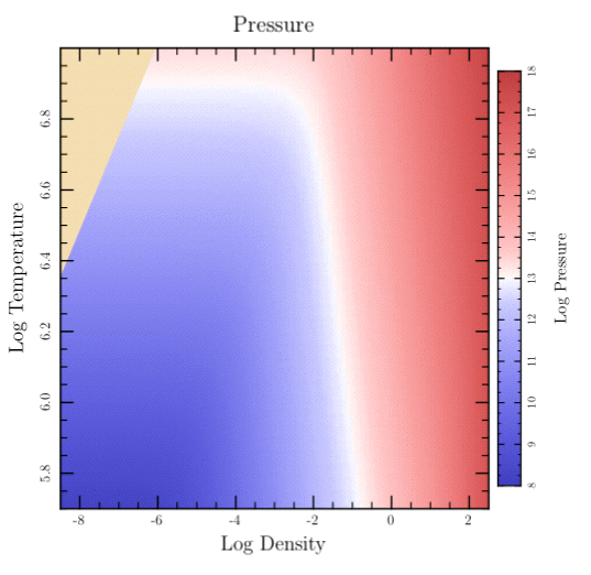
The following is a more lengthy example showing the use of a "false colored" image to represent a 2 dimensional table of data. In this case, the data comes from an astrophysical "equation of state" code that gives pressure as a function of temperature and density. The data is read from a file (using Dtable.read), converted to image samples (by create_image_data), and displayed (by show_image) using one of the predefined colormaps (mellow_colormap). Since there is no data for the high-temperature and low-density corner, that area is removed by a clip path (see the clip_press_image method below). Finally, a color bar is added showing the values for the different colors used in the image. The top-level plot method is 'sampled_data' which shows the image in one subplot and the colorbar in another.

TODO: update with a code snippet.